One post tagged with "propagation"

This post is a (hopefully quick) guide on the most important equations for computing free space propagation of a wavefront in the Fresnel regime, and how to do it properly.

Helmholtz equation and elementary waves​

First, some background. Consider a monochromatic wave $\psi$ in vacuum. It is governed by Helmholtz equation:

$$\nabla^2\psi + k^2 \psi = 0$$

where $k = 2 \pi / \lambda$ is the wavenumber. The solutions to this equation are called elementary waves, which can either be

• plane waves:

$$\psi(\mathbf{r}) = A \exp{(-j \mathbf{k} \cdot \mathbf{r})} = A \exp{[-j (k_x x + k_y y + k_z z)]}$$

• or spherical waves:

$$\psi(\mathbf{r}) = \frac{A}{r} \exp{(-j k r)}$$

The names indicate that the wavefronts (i.e. the surfaces of constant phase) are either planes or spheres. The term before the exponential is referred to as the amplitude of the wave, whereas the imaginary argument of the exponent is named the phase. For a spherical wave, the amplitude is modulated by the distance from the source due to the $1/r$ term.

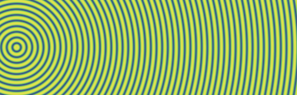
The figure below illustrates the propagation of a spherical wave. As we will understand ahead, near the source, the wavefronts are spherical. At small angles with the propagation axis, it can eventually be approximated by paraboloids. For large distances, one may approximate them by planes waves.

In the real world, though, there is no free lunch. We usually encounter waves that are way more complex than these elementary waves. Fortunately, we can make things easier using the Angular Spectrum of waves.

Angular Spectrum Method (ASM)​

An arbitrary wavefront $\psi(x_1,y_1)$ at plane $z=0$ can be decomposed into plane wave components using the Fourier transform (FT):

$$\psi(x_1,y_1) = \frac{1}{2 \pi} \iint \hat{\psi}(k_x,k_y) e^{[-j (k_x x_1 + k_y y_1)]} dk_x dk_y$$

In other words, the wavefront is composed by a sum of plane waves with phase $\phi = k_x x_1 + k_y y_1$, each with amplitude $\hat{\psi}(k_x,k_y)$. Any wavefront can be decomposed in such fashion, which makes things easier.

Now, how can one obtain the wavefront at a different plane $(x_2,y_2,z)$ in space? Well, instead of working directly with $\psi(x_1,y_1)$, one can propagate each plane wave component separately and then sum the contribution of all these elementary waves at $z$. This is done using the free space propagator:

$$H(k_x,k_y)=\exp{(j z \sqrt{k^2 - k_x^2 - k_ y^2})}$$

such that the resulting wave is

$$\psi(x_2,y_2,z) = \frac{1}{2 \pi} \iint \underbrace{\hat{\psi}_1(k_x,k_y) \exp{(j z \sqrt{k^2 - k_x^2 - k_ y^2}})}_{\text{free space propagator multiplies each component}} e^{-j (k_x x_2 + k_y y_2)}dk_x dk_y$$

This expression can be written in operator form as

$$\psi(x_2,y_2,z) = \mathcal{F}^{-1}\{ \mathcal{F}\{\psi(x_1,y_1)\} H(k_x,k_y) \}$$

The above expression arises directly from the Raleigh-Sommerfeld diffraction solution (see reference [4] for a more detailed explanation). The only assumption here is that the distance between source and observation points be much greater than the wavelength $\lambda$.

Important approximations​

We can apply approximations to get simpler forms of the propagator. For that, we make use of the paraxial approximation. It is common to hear that such approximation means the wave makes small angles with the optical axis. However, a wave may have plane wave components spreading in all directions. Hence, a more correct way of saying this is that the non-negligible plane wave components make a small angle with the optical axis [2]. A paraxial wave can also be thought as one that varies much more in the trasversal $x,y$ plane than in the longitudinal $z$ direction.

The paraxial Helmholtz equation governs paraxial waves, and it presents two important solutions:

• Paraboloidal wave

This is also known as the Fresnel diffraciton integral. It is the paraxial approximation to the spherical wave:

$$\psi(x_2,y_2) = \frac{e^{ikz}}{i \lambda z} \iint_{-\infty}^{+\infty} \psi(x_1,y_1) e^{ \frac{i k}{2 z}\left[{(x_2-x_1)^2+(y_2-y_1)^2} \right]} dx_1 dy_1$$

In this case, we have a plane wave component from the $e^{ikz}$ term which gets modulated by the phase term inside the integral. Note that $(x^2+y^2)/z = \text{const}$ is the equation of the paraboloid of revolution. Hence, the plane waves get "distorted" into paraboloids. For large distances $z$, this phase term become negligible. Also, the variation of the amplitude with the term $1/z$ becomes less relevant, which justifies the approximation of a spherical wave by a plane wave.

• Gaussian beam:

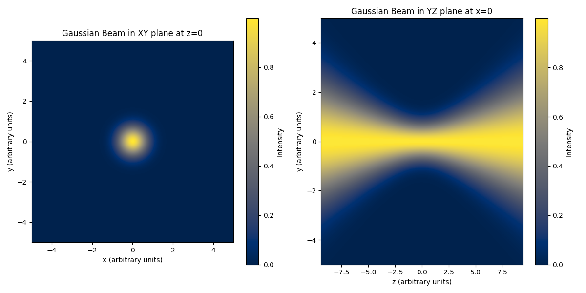
The Gaussian beam is a more complex, but extremely useful solution which appears in lasers, optical communication and many optical instruments. It is described by:

$$\psi(x, y, z) = \psi_0 \frac{w_0}{w(z)} \exp\left(-\frac{x^2 + y^2}{w(z)^2}\right) \exp\left(-ikz - ik\frac{x^2 + y^2}{2R(z)} + i\zeta(z)\right)$$

If we calculate the intensity $I=|\psi(x,y,z)|^2$, we get

$$I(x,y,z) = |\psi_0|^2 \frac{w_0^2}{w(z)^2} \exp\left(-2\frac{x^2 + y^2}{w(z)^2}\right)$$

The $xy$ dependence of the intensity is Gaussian, which explains the name. We can see the transversal slice $I(x,y)$ at $z=0$ in the figure below, which shows exactly such Gaussian distribution.

As the equation shows, there are a few parameters to model the bahavior of a Gaussian beam. First, it is useful to define the Rayleigh length $z_R$

$$z_R = \frac{\pi w_0^2}{\lambda}$$

where $w_0$ is called the beam waist, which corresponds to the minimum radius of the beam, chosen to be at $z=0$. The Rayleigh length is used to write the other quantities of interest, namely:

• Beam radius:

$$w(z) = w_0 \sqrt{1 + \left(\frac{z}{z_R}\right)^2}$$

• Radius of curvature:

$$R(z) = z \left[1 + \left(\frac{z_R}{z}\right)^2\right]$$

• Gouy phase:

$$\zeta(z) = \arctan\left(\frac{z}{z_R}\right)$$

A few comments on these equations to help us better understand the Gaussian beam:

• The transversal size of the beam is indeed minimum at $w(z=0) = w_0$. This size increases in both $\pm z$ directions. The length from $-z_R$ to $z_R$ is defined to be the depth of focus $b$ of the beam.

• The Gouy phase represents a phase delay from $-\pi/2 to \pi/2$. If we combine two of the phase terms, we have $i(kz-\zeta(z) )$. Hence, it can be understood as a phase deviation from the plane wave scenario.

• The third phase term relates to the radius of curvature, which causes the wavefront to curve. $R(z)$ is infinite at $z=0$, meaning we have a plane wave. The curvature then decreases up to a minimum at $z=z_R$. It then increases again to assimptoticaly reach $R(z)\approx z$ for big $z$. A good enough approximation is to use $R(z>2z_R) = z$.

Using the Fresnel diffraction integral​

Let us rewrite the Fresnel diffraction integral:

$$\psi(x_2,y_2) = \frac{e^{ikz}}{i \lambda z} \iint_{-\infty}^{+\infty} \psi(x_1,y_1) e^{ \frac{i k}{2 z}\left[{(x_2-x_1)^2+(y_2-y_1)^2} \right]} dx_1 dy_1 \tag{1}$$

We can expand the exponent inside the integral and move some terms out, arriving at the following form:

$$\psi(x_2,y_2) = \frac{e^{ikz}}{i \lambda z} e^{ \frac{i k}{2 z}\left[{x_2^2+y_2^2} \right]} \iint_{-\infty}^{+\infty} \psi (x_1,y_1) e^{ \frac{i k}{2 z} \left[{x_1^2+y_1^2} \right] } e^{ \frac{i k}{2 z}{(x_2 x_1+y_2 y_1)} }dx_1 dy_1 \tag{2}$$

The two approaches are named the Convolution and Fourier Transform forms of the Fresnel Diffraction integral. Although mathematically identical, they are numerically different. One must be careful to choose between them depending on the problem at hand.

Convolution form​

- Impulse Response method​

A convolution between two functions f and g is defined by

$$f \ast g = \int_{-\infty}^{+\infty} f(t) g(t-\tau) d\tau$$

Equation (1) is nothing more than a convolution of $\psi$ with the following impulse response function $h(x,y)$:

$$h(x,y) = \frac{e^{ikz}}{i \lambda z} e^{ \frac{i k}{2 z}\left[{x^2+y^2} \right]} \tag{3}$$

Hence

$$\psi(x_2,y_2) = \frac{e^{ikz}}{i \lambda z} \iint_{-\infty}^{+\infty} \psi(x_1,y_1) h(x_2-x_1,y_2-y_1) dx_1 dy_1$$

- Transfer function method​

Making use of the convolution theorem, it can be calculated in Fourier space as

$$\psi(x_2,y_2) = \mathcal{F}^{-1}\{ \mathcal{F}\{ \psi(x_1,y_1) \} H(f_{x_1},f_{y_1}) \} \tag{4}$$

where

$$H(f_{x1},f_{y1}) = \mathcal{F}\{h(x_1,y_1)\} = e^{jkz} e^{j \pi \lambda z (f_{x}^2+f_{y}^2)} \tag{5}$$

Note that in computing equation (4), one should pre-computes $H(f_{x_1},f_{y_1})$ and spares one calculation of the Fourier Transform.

Chirp functions​

Equations (3) and (5) define what we call a chirp function. For the IR method, the chirp function is sampled in real space:

$$C_1 = e^{ \frac{i k}{2 z} \left({x_1^2+y_1^2} \right) }$$

whereas for the SFT it is samples in reciprocal space:

$$C_2 = e^{j \pi \lambda z (f_{x}^2+f_{y}^2)}$$

This is the reason why they are numerically different. Correctly evaluation of the Fast Fourier transform requires proper sampling of the functions to avoid aliasing, according to the Nyquist sampling theorem. Now, the discrete Fourier Transform imposes that

$$\Delta x = \frac{1}{N \Delta f}$$

where $N$ is the number of points in your matrix. In other words, for a given N there is an inverse relationship between the sampling $\Delta x$ in real-space and the sampling $\Delta f$ in reciprocal space. This indicates that, the best one chirp function is sampled, the worst the other one will be. This is as strong indication that one method might be superior to the other depending on the situation.

How to choose the best method?​

Now, to the practical side of things. For selecting the best method for your application, one may use a rule of thumb in the table below (although for details I recommend taking a closer look at the references!). $L$ represents the size of the array and $D$ is width of the source field inside of it ($D<L$).

Criteria	Sampling	Comment
$\Delta x > \frac{\lambda z}{L}$	TF: oversampled.     IR: undersampled	IR method causes periodic copies. TF is the method of choice. Observation plane width will be limited to width $D + \lambda z / \Delta x$
$\Delta x = \frac{\lambda z}{L}$	both TF and IR: critical sampling	TF and IR are identical
$\Delta x < \frac{\lambda z}{L}$	TF: undersampled. IR: oversampled	It depends. Needs to evaluate if source bandwidth satisfies $B \le \frac{L}{2 \lambda z}$. If yes, use TF. Otherwise, IR may be better.

Fourier Transform form​

- Single Fourier Transform​

Equation (2), on the other hand, can be seen as a Fourier Transform:

$$\psi(x_2,y_2) = \frac{e^{ikz}}{i \lambda z} e^{ \frac{i k}{2 z}\left[{x_2^2+y_2^2} \right]} \mathcal{F}\{ \psi(x_1,y_1) e^{ \frac{i k}{2 z} \left[{x_1^2+y_1^2} \right] } \}$$

Notice that it can also be rewritten using $h(x,y)$, such that

$$\psi(x_2,y_2) = e^{ \frac{i k}{2 z}\left[{x_2^2+y_2^2} \right]} \mathcal{F}\{ \psi(x_1,y_1) h(x_1,y_1) \} \} \tag{6}$$

In contrast to equation (4), the above expression requires a single Fourier Transform computation.

Grid spacing​

In practice, we will compute the propagation on, well, a computer. In other words, we shall use discrete matrices. An important difference between the Single Fourier Trasform and Convolution methods is that the latter always involve an inverse Fourier transform, whereas the first does not. This has consequences on the final grid spacing of the resulting matrix.

If you perform an inverse Fourier transform at the end, the pixel sizes $p_1$ in the input and $p_2$ in the output fields will be the same. No problem there. However, if only forward Fourier transform is applied, the pixel sizes relate according to:

$$p_2 = \frac{\lambda z}{N p_1}$$

- Fresnel propagator in 2 steps​

One alternative to select the pixel size $p_2$ in the output plane is to perform the propagation in two steps. The idea is to first propagate the wavefront from $z_1$ to an intermediary plane $z_i$, and then from $z_i$ to the final desired plane $z_2$. We introduce a scaling parameter $m$ such that

$$p_2 = m p_1$$

It turns out that this scaling paremeter relates to the positions in the $z$ axis as

$$m = \left\lvert\frac{z_2 - z_i}{z_i - z_1} \right\rvert = \left\lvert\frac{\Delta z_2}{\Delta z_1} \right\rvert$$

In that case, the wavefront $\psi$ is obtained via

$$\begin{align*} \psi(x_2,y_2,z_2) & = \frac{z_2}{z_1} e^{j 2 \pi z/\lambda} \exp{\left( -j \frac{\pi}{\lambda z} \frac{z_1-z_2}{z_2} (x_2^2+y_2^2) \right)} \\ & \mathcal{F}^{-1}\{\exp{\left( -j\pi \lambda z \frac{z_1}{z_2}(f_{x1}^2+f_{y_1}^2)\right)} \mathcal{F}\{ \psi_1(x_1,y_1,z_1) \exp{\left( j \frac{\pi}{\lambda z}\frac{z_1-z_2}{z_1}(x_1^2+y_1^2)\right)}\}\} \end{align*}$$

But caution: the above expression presents an issue. It requires computing both chirp functions in real and reciprocal spaces. Therefore, unless working with critical sampling, the expression above will always be partly wrong due to undersampling of one of the two expressions.

Fresnel scaling theorem​

A particularly common scenario is that of divergent or cone-beam sources. In these cases, the beam divergence is quite large for the lengths of interest, such that the expansion of the beam becomes relevant.

The Fresnel diffraction integral is, naturally, still valid. Nonetheless, if we are dealing with large propagation distances and a large divergence, a beam with only microns in size may expand hundreds of times in size. Therefore, it may be necessary to work with matrix with dozens of thousands of pixels, making you calculation infeasible due to computer memory limitations.

Fortunately, there exists a clever workaround in this case, called the Fresnel Scaling Theorem (FST). Essentially, the FST states that a divergent spherical wave has an equivalent plane-wave equivalent with scaled pixels and distances.

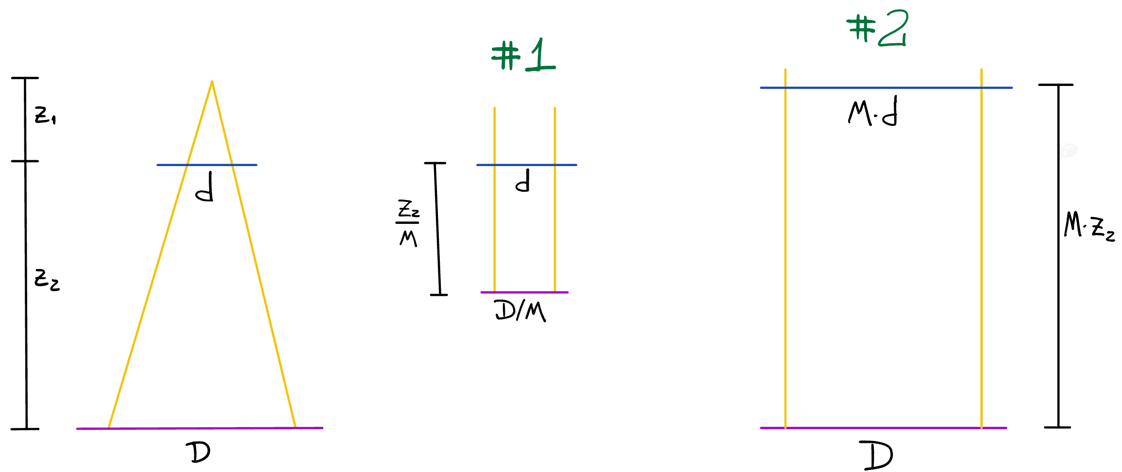
In the cone-beam case, the focus to sample distance $z_1$ and the sample to output plane distance $z_2$ define the magnification $M$ of the system:

$$M = \frac{z_1 + z_2}{z_1}$$

This quantity is used then to convert from the cone to the equivalent parallel beam geometry. Note that we recover the parallel case ($M=1$) when $z_1 \rightarrow + \infty$.

Equivalent geometry #1​

The most well know geometry puts the reference on the pixel size $d$ of the input plane. In this case, the distance between input and output planes and the output pixel size are downscaled according to

$$z_2 \rightarrow z_2/M$$

and

$$D \rightarrow D/M$$

Equivalent geometry #2​

A less well-known equivalent geometry [6] puts instead the reference on te pixel size $D$ of the output plane. In that case, an upscaling happens:

$$z_2 \rightarrow M z_2$$

and

$$D \rightarrow M D$$

Which geometry to use will depend on your specific application, whichever make your calculations easier. For a particuarly nice implementation of geometry #2, see reference [6].

Validity of the FST​

I would like to emphasize here that the Fresnel Scaling theorem assumes a point source, i.e., spherical waves. Therefore, to apply the FST the waves reaching our object in the input plane must be spherical. In many practical situations that may not be the case.

Referring back to the Gaussian beam equations, the phase is not yet spherical within the Rayleigh length. A minimum distance $2z_R$ from the beam waist is required for application of the FST, since only then the phase wavefront can be approximatted by a spherical wavefront again [7].

References​

• [1] Saleh, B. E. A., & Teich, M. C. (1991). Fundamentals of Photonics. Wiley. https://doi.org/10.1002/0471213748
• [2] Paganin, David, Coherent X-Ray Optics, Oxford Series on Synchrotron Radiation (2006), https://doi.org/10.1093/acprof:oso/9780198567288.001.0001
• [3] Goodman, J. W., & Cox, M. E. (1969). Introduction to Fourier Optics.
• [4] Voelz, D. G. (2011). Computational Fourier Optics: A MATLAB Tutorial. SPIE. https://doi.org/10.1117/3.858456
• [5] Schmidt, J. D. (2010). Numerical Simulation of Optical Wave Propagation with Examples in MATLAB. SPIE. https://doi.org/10.1117/3.866274
• [6] Hu Ziyang, et. al. (2023) “Near-Field Multi-Slice Ptychography: Quantitative Phase Imaging of Optically Thick Samples with Visible Light and X-Rays.”. https://doi.org/10.1364/OE.487002.
• [7] Robisch, Anna-Lena. “Phase Retrieval for Object and Probe in the Optical Near-Field.” Universitätsverlag Göttingen, 2016.